Foundations of Machine Learning

Examination of the end-to-end process of developing, training, testing, deploying, and monitoring machine learning systems, with focus on data quality, generative AI tools, human labour in data preparation, basic evaluation measures, and observed production failure patterns.

Overview

This lesson examines the end-to-end process of building and maintaining machine learning systems in production. It covers the development pipeline from problem definition through data preparation, model training, pre-deployment testing at multiple levels, deployment, and continuous monitoring. Central attention is given to data types and quality attributes, the extensive manual labour required for data annotation and cleaning, basic evaluation measures including error metrics and fairness notions, generative machine learning tools such as large language models and diffusion-based image generators, the full machine learning system lifecycle as a feedback loop, and recurring failure modes in deployed systems such as data drift, concept drift, adversarial attacks, and training-serving skew. The material emphasizes that reliable production performance depends primarily on systematic data handling, rigorous validation, operational monitoring, and awareness of documented practical failure patterns rather than on model architecture alone.

Learning Objectives

• Describe stages in the development, training, and deployment of machine learning systems.
• Identify testing approaches applied before deploying machine learning models.
• Classify data types and list quality attributes required for effective machine learning performance.
• Outline core capabilities and limitations of generative machine learning tools, including large language models and diffusion-based image generators.
• Map the lifecycle of a machine learning system from initial problem formulation through post-deployment monitoring.
• Explain forms of data work and associated invisible labour in machine learning development.
• Define basic evaluation concepts, including error types and fairness measures.
• List documented failure modes in deployed machine learning systems.

Motivation

Machine learning systems require coordinated processes beyond algorithm selection. Data quality, testing rigor, ongoing monitoring, and recognition of human contributions determine whether models deliver reliable results in production. Understanding these elements reduces deployment risks and supports responsible system design.

Development, Training, and Deployment of Machine Learning Systems

Development follows an iterative pipeline with interconnected stages.

1. Problem framing translates business needs into machine learning objectives.
2. Data acquisition gathers raw sources.
3. Preprocessing cleans and transforms data.
4. Feature engineering constructs predictive variables.
5. Model selection and training optimize parameters on prepared data.
6. Evaluation measures performance on held-out sets.
7. Deployment integrates the model into the production infrastructure.
8. Monitoring tracks real-world behaviour.

Training pipelines automate data flow, hyperparameter search, and version control. Deployment options include batch inference, real-time serving via APIs, or embedded models on edge devices. Containerization and orchestration tools support scalable inference.

The process follows established iterative frameworks for machine learning projects.

Figure 1: End-to-End Machine Learning Lifecycle

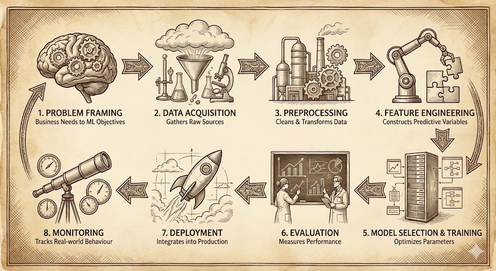
Figure 1 presents a standard end-to-end machine learning lifecycle diagram, showing stages from data collection through modeling, deployment, and monitoring in a production context.

Practical Example: Spam Email Classifier

Consider the development of a spam email classifier for an email service provider. The stages map to the pipeline as follows.

1. Problem framing: The business need is to reduce user exposure to unsolicited emails. The machine learning objective is to classify incoming emails as spam or not-spam with high precision to minimize false positives.

2. Data acquisition: Gather emails from public datasets such as Enron or SpamAssassin corpora, supplemented with labeled examples from the provider’s historical data (with user consent and anonymization).

3. Preprocessing: Remove HTML tags, convert text to lowercase, tokenize words, remove stop words, and handle attachments or links.

4. Feature engineering: Compute term frequency-inverse document frequency (TF-IDF) vectors, add features like sender domain reputation, email length, and presence of certain keywords.

5. Model selection and training: Select a logistic regression or random forest classifier. Train on a split dataset using cross-validation to optimize hyperparameters such as regularization strength.

6. Evaluation: Measure accuracy, precision, recall, and F1-score on a validation set. Ensure a low false positive rate.

7. Deployment: Integrate the model into the email server using a framework like TensorFlow Serving or MLflow for real-time classification of incoming emails.

8. Monitoring: Track classification accuracy over time, monitor for drift in email patterns (e.g., new spam tactics), and log misclassifications for periodic retraining.

Explosive growth driven by deep neural networks, large datasets, GPU acceleration, and massive compute resources. Breakthroughs in vision (2012), games (2016), and language (2018–2026). Sustained investment and rapid progress continue into 2026 with foundation models and multimodal systems.

Testing Machine Learning Systems Before Deployment

Testing machine learning systems before deployment occurs at multiple levels to ensure reliability, correctness, performance, and safety. Each level targets different aspects of the system.

Unit Tests

Verify individual components in isolation.

• Checks correctness of small, independent pieces such as data loaders, preprocessing functions, custom loss functions, or metric calculations.
• Example: Confirm that a data loader correctly reads CSV files, handles missing values as specified, and returns batches of the expected shape.

Integration Tests

Validate that components work together as a complete pipeline.

• Run end-to-end execution from raw data input to model output.
• Example: Feed a small sample dataset through the full pipeline (preprocessing → feature engineering → model inference) and assert that no errors occur and outputs match expected formats.

Performance Tests

Evaluate predictive quality on held-out validation data.

• Measure standard metrics: accuracy, precision, recall, F1-score, AUC-ROC, mean absolute error, etc.
• Example: On a validation set, confirm the model achieves at least 92% F1-score for a binary classification task and that precision exceeds 95% to minimize false positives.

Robustness Tests

Assess behavior under challenging or unexpected inputs.

• Test with noisy data, distributional shifts (e.g., covariate shift), or adversarial examples.
• Example: Add Gaussian noise to images or perturb text with typos/synonyms and measure how much performance drops; or use adversarial attack libraries (e.g., Foolbox) to generate small changes that fool the model.

Fairness Audits

Examine whether the model treats protected groups equitably.

• Check for disparate impact, demographic parity, equalized odds, or calibration across groups (e.g., gender, race, age).
• Example: Compare true positive rates and false positive rates for loan approval across ethnic groups; flag if one group has 20% lower approval rate despite similar credit scores.

Stress Tests

Measure system behavior under high load or resource constraints.

• Evaluate latency, throughput (predictions per second), memory usage, and stability during peak traffic.
• Example: Simulate 10,000 concurrent inference requests and verify that average latency stays below 200 ms and no requests time out under maximum expected load.

A/B Testing (or Online Experiments)

Compare model variants in a live production environment before full rollout.

• Route a small percentage of traffic (e.g., 5–10%) to a new model while the remainder uses the current version.
• Measure business metrics (e.g., click-through rate, conversion, user satisfaction) to decide whether to promote the new model.
• Example: Test a new recommendation model on 10% of users for two weeks; if it increases average session duration by a statistically significant 8% without raising bounce rate, proceed to full deployment.

Thorough multi-level testing reduces the risk of deploying unreliable or harmful models. In practice, combine offline evaluation (validation sets, robustness/fairness audits) with controlled online experiments (A/B testing) before granting full production access.

Types and Quality Attributes of Data

Data used in machine learning systems can be classified by structure and measurement scale. Data quality directly influences model performance: poor quality leads to unreliable predictions, amplified biases, and reduced generalization.

Data Types by Structure

Type	Description	Examples	Typical Use in ML
Structured	Organized in fixed rows and columns with clear schema	Tabular data (CSV, Excel, databases)	Customer records, sensor readings, sales transactions
Unstructured	No predefined format or schema	Text documents, images, audio, video	Social media posts, X-rays, speech recordings, surveillance footage
Semi-structured	Flexible schema with tags or key-value pairs	JSON, XML, log files, NoSQL documents	API responses, web server logs, configuration files

Measurement Scales (Data Attributes)

Scale	Category	Description	Examples	Allowed Operations
Quantitative	Discrete	Countable whole numbers	Number of children, product quantity, star ratings (1–5)	Count, add, subtract (no meaningful fractions)
Quantitative	Continuous	Real numbers with infinite possible values	Height, temperature, price in dollars	Add, subtract, multiply, divide, meaningful averages
Qualitative	Nominal	Unordered categories	Color (red, blue), city name, blood type	Equality check, count frequencies
Qualitative	Ordinal	Ordered/ranked categories without equal intervals	Education level (high school, bachelor, master), satisfaction (poor, fair, good, excellent)	Order comparison, median, rank-based stats
Qualitative	Binary	Exactly two possible states	Yes/No, true/false, 0/1, spam/not-spam	Equality, count proportions

Data Quality Attributes (Dimensions)

Quality Dimension	Description	Impact of Poor Quality	Detection / Improvement Methods
Accuracy	Data values correctly represent real-world facts (match ground truth)	Wrong predictions, misleading insights	Cross-check with trusted sources, manual validation
Completeness	No missing values or records where they are expected	Biased models (e.g., ignoring underrepresented groups)	Fill missing values, imputation, remove incomplete rows
Consistency	Uniform format, coding, and logic across the dataset	Errors in feature engineering, conflicting rules	Standardize formats, resolve contradictions
Timeliness	Data is up-to-date and relevant for the current task	Outdated patterns lead to concept drift	Set refresh schedules, use recent data windows
Validity	Values conform to defined rules, ranges, or formats	Invalid entries cause crashes or noise	Schema validation, range checks, regex patterns
Uniqueness	No unintended duplicates (each entity appears once)	Inflated importance of repeated records	Deduplication, primary key enforcement

High-quality data across these dimensions reduces bias amplification, improves model generalization, and increases trust in production predictions. In practice, most machine learning project time is spent addressing data quality issues rather than tuning models.

Introduction to Generative AI Tools

Generative AI tools are systems that create new content by learning patterns from large amounts of existing data. After learning these patterns, they can produce original text, images, audio, video, or combinations of these. The content they generate is new, but it follows the same kinds of structures and styles found in the data they were trained on.

Text-Generating AI (Language Models)

Text-generating AI tools are designed to read, understand, and produce human language. Examples include tools such as ChatGPT, Claude, and similar AI assistants.

How they learn

These systems are trained using large collections of written material such as books, articles, websites, and code. Through training, they learn how words, sentences, and ideas usually relate to one another. They are then refined to provide clear, helpful, and safe responses.

What they can do

• Write emails, reports, stories, and other written content
  
• Summarize long documents and explain topics in simple language
  
• Translate text between different languages
  
• Assist with coding, math, and problem-solving
  
• Answer questions and maintain conversations across many subjects

Image-Generating AI

Image-generating AI tools create images based on written descriptions. Popular examples include systems such as DALL·E and Stable Diffusion.

How they generate images

These tools are trained on large numbers of images and learn common visual patterns. When given a text prompt, they generate an image that matches the description by progressively refining visual details.

What they can do

• Create images from text descriptions
  
• Edit images by changing or filling in parts of an existing picture
  
• Produce artwork in different visual styles
  
• Generate high-quality images for creative, educational, or professional use

The Big Picture

Different generative AI tools specialize in different types of content: - Language models focus on text, conversation, and reasoning
- Image models focus on visual creation and editing

Newer systems are beginning to combine multiple abilities into a single tool that can work with text, images, audio, and video together. These tools are changing how people create content, share ideas, and interact with digital technology.

Key Limitations and Challenges

Generative models, despite their impressive capabilities, face several fundamental limitations and challenges that affect their reliability, fairness, and practical use.

Factual Inaccuracies and Hallucinations

Models produce plausible but incorrect statements due to reliance on statistical patterns rather than verified knowledge.

Example: When asked “Which country won the 2026 FIFA World Cup?”, a model might confidently respond “Brazil won the 2026 FIFA World Cup” based on patterns associating Brazil with frequent victories, even though the tournament has not yet occurred as of 2026.

Societal Biases

Outputs reflect imbalances and stereotypes present in training data across gender, race, ethnicity, and other attributes.

Example: Prompting for “a successful CEO” frequently generates images of white men in suits, while “a nurse” more often produces images of women, reproducing historical occupational gender distributions in training corpora.

Prompt Sensitivity

Results vary significantly based on prompt wording, requiring advanced prompting techniques such as few-shot examples, chain-of-thought, or role assignment.

Example: The prompt “Write a poem about a cat” yields a generic short poem, but “You are a 19th-century Romantic poet. Write a melancholic ode to a stray cat wandering moonlit streets” produces longer, more stylistic verse with elevated language and imagery.

Computational Requirements

Training demands extensive GPU resources; inference for large models requires substantial memory and time.

Example: Training a 70-billion-parameter language model can require thousands of GPU-hours on high-end clusters (e.g., 8,000 A100 GPUs for weeks), while running inference on GPT-4-class models needs at least 80 GB of VRAM for unquantized weights and can take several seconds per response without optimization.

Copyright and Ethical Issues

Generated content may reproduce protected works or mimic specific artist styles without attribution.

Example: An image generation model prompted with “in the style of Studio Ghibli” produces artwork closely resembling Hayao Miyazaki’s visual language, raising questions about whether the output infringes on copyrighted artistic expression or unfairly appropriates distinctive stylistic elements.

Evaluation Challenges

Automated metrics provide limited insight; human judgment remains necessary for assessing relevance, creativity, and quality.

Example: BLEU score for machine translation or FID for image generation correlates poorly with human perception of fluency or aesthetic appeal; a model achieving high FID may still produce artifacts humans find unnatural, requiring side-by-side human rankings or Likert-scale ratings for reliable assessment.

Practical Deployment Considerations

Production deployments of generative machine learning tools incorporate several techniques to address safety, reliability, efficiency, and traceability.

Content Filters

Prevent the generation of harmful or inappropriate material.

Example: OpenAI’s moderation API or custom classifiers scan both input prompts and generated outputs for categories such as hate speech, violence, self-harm, or sexual content. If detected, the system either blocks the request or returns a refusal message instead of completing generation.

Watermarking Techniques

Identify AI-generated media.

Example: Stable Diffusion implementations apply invisible statistical watermarks to pixel distributions during sampling (e.g., SynthID or StegaStamp methods). These patterns remain detectable by specialized decoders even after compression, cropping, or minor edits, allowing downstream platforms to flag synthetic images or text.

Retrieval-Augmented Generation (RAG)

Ground responses in current external sources.

Example: A customer support chatbot uses retrieval-augmented generation (RAG) by first querying a vector database of the company’s latest product documentation and knowledge base. Only then does the language model generate an answer conditioned on retrieved passages, reducing hallucinations about recent policy changes or product specifications.

Model Optimization Methods

Quantization, distillation, and faster decoding strategies to lower latency and resource use.

Example: A 70B-parameter model is quantized from FP16 to 4-bit integer weights using GPTQ or AWQ, reducing memory footprint from approximately 140 GB to under 40 GB. Knowledge distillation transfers capabilities to a smaller student model (e.g., 7B parameters). Speculative decoding or Medusa heads enable 2-3× faster inference by predicting multiple tokens in parallel during autoregressive generation.

These generative tools form the current leading approach in content creation and continue to advance toward multimodal systems handling text, images, audio, and video in integrated ways.

Basic Evaluation Ideas

Evaluation measures how well a machine learning model performs its task. Simple language helps explain key ideas without complex math. Focus remains on common error measures for classification and regression, plus fairness to ensure equitable treatment across groups.

Error in Classification Tasks

Classification predicts categories (e.g., spam/not spam, disease/no disease).

• Error rate (misclassification rate): fraction of wrong predictions.
  Simple formula: number of incorrect predictions divided by total predictions.
  Example: Out of 100 emails, the model labels 8 incorrectly (7 spam as not-spam, 1 not-spam as spam). Error rate = 8/100 = 0.08 or 8%.

• Accuracy: fraction of correct predictions (1 minus error rate).
  Example: In the same case, accuracy = 92/100 = 0.92 or 92%.
  Accuracy works well when classes have similar numbers of examples but misleads on imbalanced data (e.g., 99% non-spam emails; always predicting non-spam gives 99% accuracy but misses all spam).

• Precision: of the items the model labels positive, how many are actually positive?
  Helps when false positives cost a lot (e.g., wrongly flagging innocent emails as spam annoys users).
  Example: Model flags 20 emails as spam; 18 are truly spam. Precision = 18/20 = 90%.

• Recall (sensitivity): of all actual positive items, how many does the model catch?
  Important when missing positives hurts (e.g., missing cancer cases in medical screening).
  Example: 30 actual spam emails exist; model catches 18. Recall = 18/30 = 60%.

• F1 score: balances precision and recall (harmonic mean).
  Useful when both false positives and false negatives matter equally, especially with imbalanced data.
  Example: Precision 90%, recall 60% → F1 ≈ 72%. Higher F1 indicates better balance.

Error in Regression Tasks

Regression predicts continuous numbers (e.g., house price, temperature).

• Mean Squared Error (MSE): average of squared differences between predicted and actual values.
  Punishes large errors more (squares them).
  Example: Predicting house prices: errors of $10k, $20k, $5k → squared errors 100M, 400M, 25M → MSE = (525M)/3 ≈ 175M (in dollars squared).

• Mean Absolute Error (MAE): average of absolute differences.
  Easier to interpret in original units; treats all errors equally.
  Example: Same prices: absolute errors $10k, $20k, $5k → MAE = $11.67k.

MAE suits cases where all errors cost similarly; MSE fits when large errors should penalize more heavily.

Fairness Measures

Fairness checks whether the model treats different groups (e.g., by gender, race, age) equitably. Accuracy alone hides unequal performance.

• Demographic parity (statistical parity): positive prediction rates should be similar across groups.
  Example: Loan approval model approves 40% of male applicants and 15% of female applicants despite similar creditworthiness. This violates demographic parity (unequal approval rates), potentially discriminating against women even if overall accuracy is high.

• Equalized odds: true positive rates and false positive rates should match across groups.
  Example: Hiring model correctly identifies qualified candidates at 80% for majority group but only 50% for minority group (lower true positive rate), and wrongly rejects unqualified majority candidates at 10% but minority at 30% (higher false positive rate). This violates equalized odds, meaning the model disadvantages the minority group in both acceptance and rejection.

Practical Example: Credit Risk Model

A bank uses a model to approve loans (positive = approve).

• Overall accuracy: 85% (seems good).
• But broken down:
  • Group A (majority): 90% accuracy, 80% true positive rate (catches good borrowers), 10% false positive rate.
    
  • Group B (minority): 75% accuracy, 60% true positive rate, 25% false positive rate.
    → Equalized odds violated (different error rates across groups).
    → Demographic parity violated if approval rate 45% for Group A but 25% for Group B.
    → Model appears accurate overall but unfairly denies creditworthy applicants from Group B more often.

Evaluation extends beyond accuracy to include fairness and robustness. Accuracy alone can mask problems; combining error metrics with fairness checks ensures models perform reliably and equitably in real-world use.

Data Work and Invisible Labour in Machine Learning

Data preparation consumes the majority of time and effort in most machine learning projects, yet much of this labour remains invisible in final model descriptions, research papers, and product narratives. The work involves repetitive, low-paid, and often emotionally taxing tasks performed by humans that directly enable model performance.

Annotation

Human annotators create ground-truth labels required for supervised learning.

Example: For a computer vision model detecting skin cancer in dermatology images, annotators (often medical students or trained crowdworkers) examine thousands of skin lesion photos and draw precise bounding boxes or segmentation masks around malignant regions, assign severity grades, or classify lesion types. Each image may require multiple annotators for consensus, taking 2–10 minutes per image depending on complexity.

Transcription and Speech Annotation

Converting audio to text or labeling speech segments for speech recognition and voice assistants.

Example: Workers listen to hours of recorded customer service calls, doctor-patient conversations, or accented English speech and transcribe every word verbatim, mark speaker turns, note timestamps for disfluencies (uh, um), and flag background noise or overlapping speech. This supports training models like Whisper or Siri-like assistants, but workers frequently encounter sensitive content (medical diagnoses, personal arguments, trauma disclosures).

Moderation and Content Filtering

Reviewing and labeling harmful, toxic, or illegal content during dataset curation and model fine-tuning.

Example: During reinforcement learning from human feedback (RLHF) for ChatGPT-style models, moderators read thousands of model-generated responses and rate them for toxicity, hate speech, sexual content, violence, or misinformation. They also review user prompts that attempt jailbreaks or request illegal activities. Workers often see graphic violence, child exploitation material, self-harm instructions, or extreme political rhetoric, leading to documented psychological strain.

Quality Assurance and Label Cleaning

Reviewing and correcting existing labels to reduce noise and improve dataset reliability.

Example: In a large-scale image dataset like LAION-5B (used for Stable Diffusion training), quality assurance workers examine millions of image–caption pairs to remove duplicates, incorrect captions (e.g., “cat” labeled as “dog”), NSFW content, or low-resolution images. They also flag aesthetic or semantic mismatches, ensuring the dataset is usable for high-quality generation.

Crowdworking Platforms and Conditions

Much of this labour occurs on platforms such as Amazon Mechanical Turk, Appen, Scale AI, Clickworker, Remotasks, and Telus International.

Example: A worker in the Philippines or Kenya earns $0.01–$0.10 per image annotation or $3–$8 per hour for moderation tasks. They must complete hundreds of microtasks daily to reach minimum wage equivalents, often without benefits, sick leave, or job security. Workers report burnout, exposure to disturbing material without adequate mental health support, arbitrary account suspensions, and pressure to accept low-paying batches to maintain platform ratings.

This labour is “invisible” because: - Final models and research papers rarely mention the scale of human input required. - Companies present capabilities as purely algorithmic achievements. - End-users interact with polished products without awareness of the human cost behind training data.

Recognizing this work highlights the human foundation of modern machine learning and raises questions about fair compensation, ethical sourcing, and transparency in AI development.

Failure Modes in Practice

Deployed machine learning systems exhibit recurring failure modes that degrade performance or cause unintended consequences.

Data Drift

Gradual input distribution changes degrade performance.

Example: A credit scoring model trained on 2015–2020 loan applications begins to underperform in 2025 because economic conditions, applicant demographics, and income distributions have shifted due to inflation, remote work trends, and policy changes, leading to higher default prediction errors.

Concept Drift

Target variable relationships evolve.

Example: A fraud detection model for online transactions misclassifies legitimate purchases as fraudulent after a major e-commerce platform introduces one-click checkout with biometric authentication. The relationship between transaction features (time, location, amount) and fraud label changes, rendering old patterns obsolete.

Model Decay

Accuracy drops over time without explicit shifts.

Example: A product recommendation system on an e-commerce site sees a steady decline in click-through rate over 18 months. No sudden data or concept shift occurs, but gradual changes in user preferences, seasonal effects, and catalog updates accumulate to erode relevance of recommendations trained on older behavior.

Adversarial Inputs

Small perturbations cause misclassification.

Example: An autonomous vehicle’s object detection model fails to recognize a stop sign when small adversarial stickers are placed on it. The perturbations are imperceptible to humans but cause the model to classify the sign as a 45 km/h speed limit sign, potentially leading to a traffic violation or accident.

Feedback Loops

Model outputs influence future data collection.

Example: A job recommendation algorithm on a hiring platform disproportionately recommends high-paying roles to candidates from certain universities. Over time, applicants from those universities receive more interviews and offers, reinforcing the bias in future training data and amplifying the disparity.

Infrastructure Mismatches

Training and serving environments differ.

Example: A model trained with floating-point 32-bit precision on GPU achieves high accuracy in development. When deployed on CPU-based edge devices using integer quantization without proper calibration, rounding errors accumulate and cause systematic performance degradation in real-time inference.

Silent Failures

Predictions appear valid but produce harmful downstream effects.

Example: A medical triage chatbot correctly classifies symptoms as low-risk but fails to detect subtle patterns indicative of rare conditions. The output appears reasonable (no urgent referral), but the patient delays seeking care, leading to worsened outcomes without triggering any obvious error flag.

Monitoring systems must detect these patterns early through statistical tests on input distributions, performance tracking on holdout or shadow data, anomaly detection on prediction confidence, and periodic human review of edge cases.

Summary

Machine learning systems depend on structured pipelines from problem framing to continuous monitoring. Data quality and human annotation labour underpin performance. Generative tools expand capabilities while introducing specific risks. Evaluation extends beyond accuracy to include fairness and robustness. Production failures often stem from temporal changes and distributional mismatches rather than model architecture alone.